
Configuring and Verifying EIGRP in an Enterprise WAN
![]() This section provides insight into EIGRP deployment over various WAN technologies including physical Frame Relay, multipoint and point-to-point Frame-Relay subinterfaces, Multiprotocol Label Switching (MPLS) virtual private networks (VPNs), and Ethernet over Multiprotocol Label Switching (EoMPLS). Advanced configuration options for EIGRP load balancing and limiting EIGRP bandwidth utilization on WAN links are also explored.
This section provides insight into EIGRP deployment over various WAN technologies including physical Frame Relay, multipoint and point-to-point Frame-Relay subinterfaces, Multiprotocol Label Switching (MPLS) virtual private networks (VPNs), and Ethernet over Multiprotocol Label Switching (EoMPLS). Advanced configuration options for EIGRP load balancing and limiting EIGRP bandwidth utilization on WAN links are also explored.
 EIGRP over Frame Relay and on a Physical Interface
![]() This section reviews Frame Relay and describes how EIGRP can be deployed over Frame Relay physical interfaces.
This section reviews Frame Relay and describes how EIGRP can be deployed over Frame Relay physical interfaces.
Frame Relay Overview
![]() Frame Relay is a switched WAN technology where virtual circuits (VCs) are created by a service provider (SP) through the network. Frame Relay allows multiple logical VCs to be multiplexed over a single physical interface. The VCs are typically PVCs that are identified by a data-link connection identifier (DLCI). DLCIs are locally significant between the local router and the Frame Relay switch to which the router is connected. Therefore, each end of the PVC may have a different DLCI. The SP’s network takes care of sending the data through the PVC. To provide IP layer connectivity, a mapping between IP addresses and DLCIs must be defined, either dynamically or statically.
Frame Relay is a switched WAN technology where virtual circuits (VCs) are created by a service provider (SP) through the network. Frame Relay allows multiple logical VCs to be multiplexed over a single physical interface. The VCs are typically PVCs that are identified by a data-link connection identifier (DLCI). DLCIs are locally significant between the local router and the Frame Relay switch to which the router is connected. Therefore, each end of the PVC may have a different DLCI. The SP’s network takes care of sending the data through the PVC. To provide IP layer connectivity, a mapping between IP addresses and DLCIs must be defined, either dynamically or statically.
![]() By default, a Frame Relay network is an NBMA network. In an NBMA environment all routers are on the same subnet, but broadcast (and multicast) packets cannot be sent just once as they are in a broadcast environment such as Ethernet.
By default, a Frame Relay network is an NBMA network. In an NBMA environment all routers are on the same subnet, but broadcast (and multicast) packets cannot be sent just once as they are in a broadcast environment such as Ethernet.
![]() To emulate the LAN broadcast capability that is required by IP routing protocols (for example, to send EIGRP hello or update packets to all neighbors reachable over an IP subnet), the Cisco IOS implements pseudo-broadcasting, in which the router creates a copy of the broadcast or multicast packet for each neighbor reachable through the WAN media, and sends it over the appropriate PVC for that neighbor.
To emulate the LAN broadcast capability that is required by IP routing protocols (for example, to send EIGRP hello or update packets to all neighbors reachable over an IP subnet), the Cisco IOS implements pseudo-broadcasting, in which the router creates a copy of the broadcast or multicast packet for each neighbor reachable through the WAN media, and sends it over the appropriate PVC for that neighbor.
![]() In environments where a router has a large number of neighbors reachable through a single WAN interface, pseudo-broadcasting has to be tightly controlled because it could increase the CPU resources and WAN bandwidth used. Pseudo-broadcasting can be controlled with the broadcast option on static maps in a Frame Relay configuration. However, pseudo-broadcasting cannot be controlled for neighbors reachable through dynamic maps created via Frame Relay Inverse Address Resolution Protocol (ARP). Dynamic maps always allow pseudo-broadcasting.
In environments where a router has a large number of neighbors reachable through a single WAN interface, pseudo-broadcasting has to be tightly controlled because it could increase the CPU resources and WAN bandwidth used. Pseudo-broadcasting can be controlled with the broadcast option on static maps in a Frame Relay configuration. However, pseudo-broadcasting cannot be controlled for neighbors reachable through dynamic maps created via Frame Relay Inverse Address Resolution Protocol (ARP). Dynamic maps always allow pseudo-broadcasting.
![]() Frame Relay neighbor loss is detected only after the routing protocol hold time expires or if the interface goes down. An interface is considered to be up as long as at least one PVC is active.
Frame Relay neighbor loss is detected only after the routing protocol hold time expires or if the interface goes down. An interface is considered to be up as long as at least one PVC is active.
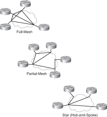
![]() Frame Relay allows remote sites to be interconnected using full-mesh, partial-mesh, and hub-and-spoke (also called star) topologies, as shown in Figure 2-23.
Frame Relay allows remote sites to be interconnected using full-mesh, partial-mesh, and hub-and-spoke (also called star) topologies, as shown in Figure 2-23.
EIGRP on a Physical Frame Relay Interface with Dynamic Mapping
![]() To deploy EIGRP over a physical interface using Inverse ARP dynamic mapping is easy because it is the default. Figure 2-24 illustrates an example network. Example 2-27 is the configuration of Router R1 in the figure. The physical interface Serial 0/0 is configured for Frame Relay encapsulation and an IP address is assigned. Inverse ARP is on by default and will automatically map the IP addresses of the devices at the other ends of the PVCs to the local DLCI number. EIGRP is enabled using autonomous system number 110, and the proper interfaces and networks are included in EIGRP using the network commands under the EIGRP routing process.
To deploy EIGRP over a physical interface using Inverse ARP dynamic mapping is easy because it is the default. Figure 2-24 illustrates an example network. Example 2-27 is the configuration of Router R1 in the figure. The physical interface Serial 0/0 is configured for Frame Relay encapsulation and an IP address is assigned. Inverse ARP is on by default and will automatically map the IP addresses of the devices at the other ends of the PVCs to the local DLCI number. EIGRP is enabled using autonomous system number 110, and the proper interfaces and networks are included in EIGRP using the network commands under the EIGRP routing process.


encapsulation frame-relay
ip address 192.168.1.101 255.255.255.0
!
router eigrp 110
network 172.16.1.0 0.0.0.255
network 192.168.1.0
![]() Split horizon is disabled by default on Frame Relay physical interfaces. Therefore, routes from Router R2 can be sent to Router R3, and vice versa. Note that Inverse ARP does not provide dynamic mapping for the communication between Routers R2 and R3 because they are not connected with a PVC. You must configure this mapping manually.
Split horizon is disabled by default on Frame Relay physical interfaces. Therefore, routes from Router R2 can be sent to Router R3, and vice versa. Note that Inverse ARP does not provide dynamic mapping for the communication between Routers R2 and R3 because they are not connected with a PVC. You must configure this mapping manually.
![]() The sample outputs of the show ip eigrp neighbors command in Example 2-28 show the neighbors of Routers R1 and R3. Router R1 forms the adjacency with Router R2 and R3 over the Serial 0/0 physical interface. Likewise, Router R3 (and R2) forms an adjacency with Router R1. In this example, no EIGRP relationship exists between Routers R2 and R3.
The sample outputs of the show ip eigrp neighbors command in Example 2-28 show the neighbors of Routers R1 and R3. Router R1 forms the adjacency with Router R2 and R3 over the Serial 0/0 physical interface. Likewise, Router R3 (and R2) forms an adjacency with Router R1. In this example, no EIGRP relationship exists between Routers R2 and R3.
IP-EIGRP neighbors for process 110
H Address Interface Hold Uptime SRTT RTO Q Seq
(sec) (ms) Cnt Num
0 192.168.1.102 Se0/0 10 00:07:22 10 2280 0 5
1 192.168.1.103 Se0/0 10 00:09:34 10 2320 0 9
R3#show ip eigrp neighbors
IP-EIGRP neighbors for process 110
H Address Interface Hold Uptime SRTT RTO Q Seq
(sec) (ms) Cnt Num
0 192.168.1.101 Se0/0 10 00:11:45 10 1910 0 6
EIGRP on a Frame Relay Physical Interface with Static Mapping
![]() To deploy EIGRP over the physical interface on Router R1 using static mapping, thus disabling the Inverse ARP, no changes are needed to the basic EIGRP configuration. Example 2-29 illustrates the configuration on Routers R1 and R3. EIGRP is enabled using autonomous system number 110, and the proper interfaces and networks are included in EIGRP using the network commands under the EIGRP routing process. Manual IP-to-DLCI mapping commands on the serial 0/0 interface are necessary on all three routers. (Router R2’s configuration is similar to R3’s.)
To deploy EIGRP over the physical interface on Router R1 using static mapping, thus disabling the Inverse ARP, no changes are needed to the basic EIGRP configuration. Example 2-29 illustrates the configuration on Routers R1 and R3. EIGRP is enabled using autonomous system number 110, and the proper interfaces and networks are included in EIGRP using the network commands under the EIGRP routing process. Manual IP-to-DLCI mapping commands on the serial 0/0 interface are necessary on all three routers. (Router R2’s configuration is similar to R3’s.)
![]() The frame-relay map protocol protocol-address dlci [broadcast] [ietf | cisco] [payload-compress {packet-by-packet | frf9 stac}] interface configuration command statically maps the remote router’s network layer address to the local DLCI. Table 2-6 details the parameters for this command.
The frame-relay map protocol protocol-address dlci [broadcast] [ietf | cisco] [payload-compress {packet-by-packet | frf9 stac}] interface configuration command statically maps the remote router’s network layer address to the local DLCI. Table 2-6 details the parameters for this command.
|
|
|
|---|---|
|
|
|
|
|
|
|
|
|
|
|
|
|
|
|
|
|
|
|
|
|
|
|
|
![]() Because split horizon is disabled by default on Frame Relay physical interfaces, routes from Router R2 can be sent to Router R3, and vice versa.
Because split horizon is disabled by default on Frame Relay physical interfaces, routes from Router R2 can be sent to Router R3, and vice versa.
| Note |
|
![]() Example 2-30 displays the adjacency formed between Router R1 and Routers R2 and R3 over the Serial 0/0 physical interface. The adjacencies formed on R1 using static mapping are the same as those formed using dynamic mapping. Routers R2 and R3 also form an adjacency with Router R1. Routers R2 and R3 can also form an EIGRP adjacency to each other if the IP-to-DLCI mapping for that connectivity is provided. Example 2-30 shows that Router R3 has only one neighbor, Router R1, indicating that this mapping was not provided on R3.
Example 2-30 displays the adjacency formed between Router R1 and Routers R2 and R3 over the Serial 0/0 physical interface. The adjacencies formed on R1 using static mapping are the same as those formed using dynamic mapping. Routers R2 and R3 also form an adjacency with Router R1. Routers R2 and R3 can also form an EIGRP adjacency to each other if the IP-to-DLCI mapping for that connectivity is provided. Example 2-30 shows that Router R3 has only one neighbor, Router R1, indicating that this mapping was not provided on R3.
IP-EIGRP neighbors for process 110
H Address Interface Hold Uptime SRTT RTO Q Seq
(sec) (ms) Cnt Num
0 192.168.1.102 Se0/0 10 00:06:20 10 2280 0 5
1 192.168.1.103 Se0/0 10 00:08:31 10 2320 0 9
R3#show ip eigrp neighbors
IP-EIGRP neighbors for process 110
H Address Interface Hold Uptime SRTT RTO Q Seq
(sec) (ms) Cnt Num
0 192.168.1.101 Se0/0 10 00:10:44 10 1910 0 6
EIGRP over Frame Relay Multipoint Subinterfaces
![]() This section describes how you can deploy EIGRP using Frame Relay multipoint subinterfaces and explores the use of EIGRP unicast neighbors.
This section describes how you can deploy EIGRP using Frame Relay multipoint subinterfaces and explores the use of EIGRP unicast neighbors.
Frame Relay Multipoint Subinterfaces
![]() You can create one or several multipoint subinterfaces over a single Frame Relay physical interface. These multipoint subinterfaces are logical interfaces emulating a multiaccess network. They act like an NBMA physical interface, and therefore use a single subnet, preserving the IP address space.
You can create one or several multipoint subinterfaces over a single Frame Relay physical interface. These multipoint subinterfaces are logical interfaces emulating a multiaccess network. They act like an NBMA physical interface, and therefore use a single subnet, preserving the IP address space.
![]() Frame Relay multipoint is applicable to partial-mesh and full-mesh topologies. Partial-mesh Frame Relay networks must deal with split-horizon issues, which prevent routing updates from being retransmitted on the same interface on which they were received.
Frame Relay multipoint is applicable to partial-mesh and full-mesh topologies. Partial-mesh Frame Relay networks must deal with split-horizon issues, which prevent routing updates from being retransmitted on the same interface on which they were received.
![]() EIGRP neighbor loss detection is particularly slow on multipoint subinterfaces configured over low-speed WAN links because the default values of the EIGRP timers on these interfaces are 60 seconds for the hello timer and 180 seconds for the hold timer. In the worst case, neighbor loss detection can take up to 3 minutes. Also, on Frame Relay multipoint subinterfaces, all of the PVCs attached to the subinterface must be lost for the subinterface to be declared down.
EIGRP neighbor loss detection is particularly slow on multipoint subinterfaces configured over low-speed WAN links because the default values of the EIGRP timers on these interfaces are 60 seconds for the hello timer and 180 seconds for the hold timer. In the worst case, neighbor loss detection can take up to 3 minutes. Also, on Frame Relay multipoint subinterfaces, all of the PVCs attached to the subinterface must be lost for the subinterface to be declared down.
EIGRP over Multipoint Subinterfaces
![]() Multipoint subinterfaces are configured with the interface serial number.subinterface-number multipoint command. For Frame Relay, the IP address-to-DLCI mapping on multipoint subinterfaces is done by either specifying the local DLCI value (using the frame-relay interface-dlci dlci command) and relying on Inverse ARP, or using manual IP address-to-DLCI mapping.
Multipoint subinterfaces are configured with the interface serial number.subinterface-number multipoint command. For Frame Relay, the IP address-to-DLCI mapping on multipoint subinterfaces is done by either specifying the local DLCI value (using the frame-relay interface-dlci dlci command) and relying on Inverse ARP, or using manual IP address-to-DLCI mapping.
![]() Figure 2-25 illustrates an example network. Example 2-31 illustrates the configuration of Routers R1 and R3 in the figure. The physical interface Serial 0/0 on each router is configured for Frame Relay encapsulation. The physical interface does not have an IP address assigned to it. (Note that in this example R3 only has one Frame Relay DLCI, so does not really need to be multipoint, or even a subinterface.)
Figure 2-25 illustrates an example network. Example 2-31 illustrates the configuration of Routers R1 and R3 in the figure. The physical interface Serial 0/0 on each router is configured for Frame Relay encapsulation. The physical interface does not have an IP address assigned to it. (Note that in this example R3 only has one Frame Relay DLCI, so does not really need to be multipoint, or even a subinterface.)


![]() A multipoint subinterface Serial 0/0.1 is created and an IP address is assigned to it.
A multipoint subinterface Serial 0/0.1 is created and an IP address is assigned to it.
![]() Split horizon is enabled by default on Frame Relay multipoint subinterfaces. In this example, Routers R2 and R3 need to provide connectivity between their connected networks, so EIGRP split horizon is disabled on the multipoint subinterface of Router R1 with the no ip split-horizon eigrp as-number command.
Split horizon is enabled by default on Frame Relay multipoint subinterfaces. In this example, Routers R2 and R3 need to provide connectivity between their connected networks, so EIGRP split horizon is disabled on the multipoint subinterface of Router R1 with the no ip split-horizon eigrp as-number command.
![]() Manual IP address-to-DLCI mapping is also configured, using the frame-relay map commands with the broadcast keyword.
Manual IP address-to-DLCI mapping is also configured, using the frame-relay map commands with the broadcast keyword.
![]() The EIGRP configuration is not changed from the basic deployment. In Example 2-31, EIGRP is enabled using autonomous system number 110 and the proper interfaces, and networks are included in EIGRP using the network commands under the EIGRP routing process.
The EIGRP configuration is not changed from the basic deployment. In Example 2-31, EIGRP is enabled using autonomous system number 110 and the proper interfaces, and networks are included in EIGRP using the network commands under the EIGRP routing process.
![]() Note that the Router R1 configuration includes frame-relay map command to its own IP address on the multipoint serial subinterface so that the Serial 0/0.1 local IP address can be pinged from Router R1 itself.
Note that the Router R1 configuration includes frame-relay map command to its own IP address on the multipoint serial subinterface so that the Serial 0/0.1 local IP address can be pinged from Router R1 itself.
![]() To verify the operation of the EIGRP routing protocol over Frame Relay multipoint subinterfaces, use the show ip eigrp neighbors command. Example 2-32 shows sample outputs for Routers R1 and R3. Router R1 forms an adjacency with Routers R2 and R3 over the serial0/0.1 multipoint subinterface. Routers R2 and R3 form the adjacency with Router R1. (R2 and R3 could also for an adjacency between each other if the IP address-to-DLCI mapping for that connectivity was provided.)
To verify the operation of the EIGRP routing protocol over Frame Relay multipoint subinterfaces, use the show ip eigrp neighbors command. Example 2-32 shows sample outputs for Routers R1 and R3. Router R1 forms an adjacency with Routers R2 and R3 over the serial0/0.1 multipoint subinterface. Routers R2 and R3 form the adjacency with Router R1. (R2 and R3 could also for an adjacency between each other if the IP address-to-DLCI mapping for that connectivity was provided.)
IP-EIGRP neighbors for process 110
H Address Interface Hold Uptime SRTT RTO Q Seq
(sec) (ms) Cnt Num
0 192.168.1.102 Se0/0.1 10 00:06:41 10 2280 0 5
1 192.168.1.103 Se0/0.1 10 00:08:52 10 2320 0 9
R3#show ip eigrp neighbors
IP-EIGRP neighbors for process 110
H Address Interface Hold Uptime SRTT RTO Q Seq
(sec) (ms) Cnt Num
0 192.168.1.101 Se0/0.1 10 00:10:37 10 1910 0 6
EIGRP Unicast Neighbors
![]() The neighbor {ip-address | ipv6-address} interface-type interface-number router configuration command is used to define a neighboring router with which to exchange EIGRP routing information. Instead of using multicast packets, EIGRP exchanges routing information with the specified neighbor using unicast packets. The router does not process any EIGRP multicast packets coming inbound on that interface and it stops sending EIGRP multicast packets on that interface. Multiple neighbor statements can be used to establish peering sessions with multiple specific EIGRP neighbors. The interface through which EIGRP will exchange routing updates must be specified in the neighbor statement. The interfaces through which two EIGRP neighbors exchange routing updates must be configured with IP addresses from the same network.
The neighbor {ip-address | ipv6-address} interface-type interface-number router configuration command is used to define a neighboring router with which to exchange EIGRP routing information. Instead of using multicast packets, EIGRP exchanges routing information with the specified neighbor using unicast packets. The router does not process any EIGRP multicast packets coming inbound on that interface and it stops sending EIGRP multicast packets on that interface. Multiple neighbor statements can be used to establish peering sessions with multiple specific EIGRP neighbors. The interface through which EIGRP will exchange routing updates must be specified in the neighbor statement. The interfaces through which two EIGRP neighbors exchange routing updates must be configured with IP addresses from the same network.
| Note |
|
![]() In Example 2-33, Router R1 (from Figure 2-25) is configured with a neighbor command for Router R2. Router R1 will therefore not accept multicast packets on Serial 0/0.1 anymore. To establish an adjacency with Router R1, Router R2 must also be configured with a neighbor command, for Router R1. R2’s configuration is provided in Example 2-34. The neighbor command enables Router R2 to use unicast packets, which will be accepted by Router R1. In this scenario, Router R3 is not configured with a neighbor command for Router R1, nor is Router R1 configured with a neighbor command for Router R3. Therefore, Router R1 and R3 will not form an adjacency.
In Example 2-33, Router R1 (from Figure 2-25) is configured with a neighbor command for Router R2. Router R1 will therefore not accept multicast packets on Serial 0/0.1 anymore. To establish an adjacency with Router R1, Router R2 must also be configured with a neighbor command, for Router R1. R2’s configuration is provided in Example 2-34. The neighbor command enables Router R2 to use unicast packets, which will be accepted by Router R1. In this scenario, Router R3 is not configured with a neighbor command for Router R1, nor is Router R1 configured with a neighbor command for Router R3. Therefore, Router R1 and R3 will not form an adjacency.
![]() To verify the EIGRP unicast neighbor configuration, use the show ip eigrp neighbors command, as shown in Example 2-35. Routers R1 and R2 have formed a neighbor relationship. The sample output does not show that the neighbor command was used on both routers, but it does indicate that a neighbor relationship is established, proof that the configuration was successfully completed.
To verify the EIGRP unicast neighbor configuration, use the show ip eigrp neighbors command, as shown in Example 2-35. Routers R1 and R2 have formed a neighbor relationship. The sample output does not show that the neighbor command was used on both routers, but it does indicate that a neighbor relationship is established, proof that the configuration was successfully completed.
![]() Because Router R3 is not using the neighbor command, it tries to communicate with multicast packets on its Serial 0/0/.1. However, neighborship is not established because neither Router R1 nor Router R2 is accepting multicast packets.
Because Router R3 is not using the neighbor command, it tries to communicate with multicast packets on its Serial 0/0/.1. However, neighborship is not established because neither Router R1 nor Router R2 is accepting multicast packets.
IP-EIGRP neighbors for process 110
H Address Interface Hold Uptime SRTT RTO Q Seq
(sec) (ms) Cnt Num
0 192.168.1.102 Se0/0/1 10 00:07:22 10 2280 0 5
R2#show ip eigrp neighbors
IP-EIGRP neighbors for process 110
H Address Interface Hold Uptime SRTT RTO Q Seq
(sec) (ms) Cnt Num
0 192.168.1.101 Se0/0/1 10 00:17:02 10 1380 0 5
EIGRP over Frame Relay Point-to-Point Subinterfaces
![]() This section describes how you can deploy EIGRP using Frame Relay point-to-point subinterfaces.
This section describes how you can deploy EIGRP using Frame Relay point-to-point subinterfaces.
Frame Relay Point-to-Point Subinterfaces
![]() One or several point-to-point subinterfaces can be created over a single Frame Relay physical interface. These point-to-point subinterfaces are logical interfaces emulating a leased line network and provide a routing equivalent to point-to-point physical interfaces. As with physical point-to-point interfaces, each interface requires its own subnet. Frame Relay point-to point is applicable to hub and spoke topologies.
One or several point-to-point subinterfaces can be created over a single Frame Relay physical interface. These point-to-point subinterfaces are logical interfaces emulating a leased line network and provide a routing equivalent to point-to-point physical interfaces. As with physical point-to-point interfaces, each interface requires its own subnet. Frame Relay point-to point is applicable to hub and spoke topologies.
![]() EIGRP neighbor loss detection is quite fast on point-to-point subinterfaces because the default values of the EIGRP hello timer and the EIGRP hold timer are identical to the values used on point-to-point physical links (5 seconds for the hello timer and 15 seconds for the hold timer). In the worst case, the neighbor loss is detected within 15 seconds. Another reason that neighbor loss is fast is that a Frame Relay point-to-point subinterface is declared down if the DLCI attached to the interface is lost—neighbor loss detection is immediate. Recall that for multipoint subinterfaces, all the PVCs attached to it must be lost for the interface to be declared down.
EIGRP neighbor loss detection is quite fast on point-to-point subinterfaces because the default values of the EIGRP hello timer and the EIGRP hold timer are identical to the values used on point-to-point physical links (5 seconds for the hello timer and 15 seconds for the hold timer). In the worst case, the neighbor loss is detected within 15 seconds. Another reason that neighbor loss is fast is that a Frame Relay point-to-point subinterface is declared down if the DLCI attached to the interface is lost—neighbor loss detection is immediate. Recall that for multipoint subinterfaces, all the PVCs attached to it must be lost for the interface to be declared down.
| Note |
|
EIGRP on Frame Relay Point-to-Point Subinterfaces
![]() Point-to-point subinterfaces are created with the interface serial number.subinterface-number point-to-point command. For Frame Relay, IP address-to-DLCI mapping on point-to-point subinterfaces is done by specifying the local DLCI value, using the frame-relay interface-dlci dlci command.
Point-to-point subinterfaces are created with the interface serial number.subinterface-number point-to-point command. For Frame Relay, IP address-to-DLCI mapping on point-to-point subinterfaces is done by specifying the local DLCI value, using the frame-relay interface-dlci dlci command.
![]() Figure 2-26 illustrates an example network; Example 2-36 is the configuration of Router R1, and Example 2-37 is the configuration of Router R3. The physical interface Serial 0/0 is configured for Frame Relay encapsulation. The physical interface does not have an IP address assigned to it.
Figure 2-26 illustrates an example network; Example 2-36 is the configuration of Router R1, and Example 2-37 is the configuration of Router R3. The physical interface Serial 0/0 is configured for Frame Relay encapsulation. The physical interface does not have an IP address assigned to it.


![]() On Router R1, two point-to-point subinterfaces, Serial 0/0.2 and Serial 0/0.3, are created and IP addresses are assigned to them. The IP address-to-DLCI mapping is provided for each subinterface. The EIGRP configuration is not changed from the basic deployment. EIGRP is enabled using autonomous system number 110 and the proper interfaces, and networks are included in EIGRP using the network commands under the EIGRP routing process.
On Router R1, two point-to-point subinterfaces, Serial 0/0.2 and Serial 0/0.3, are created and IP addresses are assigned to them. The IP address-to-DLCI mapping is provided for each subinterface. The EIGRP configuration is not changed from the basic deployment. EIGRP is enabled using autonomous system number 110 and the proper interfaces, and networks are included in EIGRP using the network commands under the EIGRP routing process.
![]() Router R3 is configured similar to Router R1, with one point-to-point subinterface. The show ip eigrp neighbors command can be used to verify the operation of the EIGRP routing protocol over the Frame Relay point-to point subinterface. Example 2-38 shows sample outputs for Routers R1 and R3. Router R1 forms the adjacency with Router R2 over its Serial 0/0.2 point-to-point interface and with Router R3 over its Serial 0/0.3 point-to-point subinterface. Likewise, Routers R2 and R3 form the adjacency with Router R1 over the Serial 0/0.1 point-to-point subinterface. Router R3 has one neighbor, Router R1, over its Serial 0/0.1 point-to-point subinterface.
Router R3 is configured similar to Router R1, with one point-to-point subinterface. The show ip eigrp neighbors command can be used to verify the operation of the EIGRP routing protocol over the Frame Relay point-to point subinterface. Example 2-38 shows sample outputs for Routers R1 and R3. Router R1 forms the adjacency with Router R2 over its Serial 0/0.2 point-to-point interface and with Router R3 over its Serial 0/0.3 point-to-point subinterface. Likewise, Routers R2 and R3 form the adjacency with Router R1 over the Serial 0/0.1 point-to-point subinterface. Router R3 has one neighbor, Router R1, over its Serial 0/0.1 point-to-point subinterface.
IP-EIGRP neighbors for process 110
H Address Interface Hold Uptime SRTT RTO Q Seq
(sec) (ms) Cnt Num
0 192.168.2.102 Se0/0.2 10 00:08:04 10 2280 0 5
1 192.168.3.103 Se0/0.3 10 00:10:12 10 2320 0 9
R3#show ip eigrp neighbors
IP-EIGRP neighbors for process 110
H Address Interface Hold Uptime SRTT RTO Q Seq
(sec) (ms) Cnt Num
0 192.168.3.101 Se0/0.1 10 00:13:25 10 1910 0 6
EIGRP over MPLS
![]() This section provides an overview of MPLS and Layer 2 and Layer 3 MPLS VPN technologies and explains how you can deploy EIGRP in such environment.
This section provides an overview of MPLS and Layer 2 and Layer 3 MPLS VPN technologies and explains how you can deploy EIGRP in such environment.
MPLS
![]() MPLS is an Internet Engineering Task Force (IETF) standard architecture that combines the advantages of Layer 3 routing with the benefits of Layer 2 switching.
MPLS is an Internet Engineering Task Force (IETF) standard architecture that combines the advantages of Layer 3 routing with the benefits of Layer 2 switching.
![]() With MPLS, short fixed-length labels are assigned to each packet at the edge of the network. Rather than examining the IP packet header information, MPLS nodes use this label to determine how to process the data.
With MPLS, short fixed-length labels are assigned to each packet at the edge of the network. Rather than examining the IP packet header information, MPLS nodes use this label to determine how to process the data.
![]() This process results in a more scalable and flexible WAN solution. The MPLS standards evolved from the efforts of many companies, including Cisco’s tag-switching technology.
This process results in a more scalable and flexible WAN solution. The MPLS standards evolved from the efforts of many companies, including Cisco’s tag-switching technology.
![]() MPLS enables scalable VPNs, end-to-end quality of service (QoS), and other IP services that allow efficient utilization of existing networks with simpler configuration, management, and quicker fault correction.
MPLS enables scalable VPNs, end-to-end quality of service (QoS), and other IP services that allow efficient utilization of existing networks with simpler configuration, management, and quicker fault correction.
MPLS Operation
![]() MPLS is a connection-oriented technology whose operation is based on a label attached to each packet as it enters the MPLS network. A label identifies a flow of packets (for example, voice traffic between two nodes), also called a forwarding equivalence class (FEC). An FEC is a grouping of packets. Packets belonging to the same FEC receive the same treatment in the network. The FEC can be determined by various parameters, including source or destination IP address or port numbers, IP protocol, IP precedence, or Layer 2 circuit identifier. Therefore, the FEC can define the flow’s QoS requirements. In addition, appropriate queuing and discard policies can be applied for FECs.
MPLS is a connection-oriented technology whose operation is based on a label attached to each packet as it enters the MPLS network. A label identifies a flow of packets (for example, voice traffic between two nodes), also called a forwarding equivalence class (FEC). An FEC is a grouping of packets. Packets belonging to the same FEC receive the same treatment in the network. The FEC can be determined by various parameters, including source or destination IP address or port numbers, IP protocol, IP precedence, or Layer 2 circuit identifier. Therefore, the FEC can define the flow’s QoS requirements. In addition, appropriate queuing and discard policies can be applied for FECs.
![]() The MPLS network nodes, called label-switched routers (LSRs), use the label to determine the next hop for the packet. The LSRs do not need to examine the packet’s IP header; rather, they forward it based on the label.
The MPLS network nodes, called label-switched routers (LSRs), use the label to determine the next hop for the packet. The LSRs do not need to examine the packet’s IP header; rather, they forward it based on the label.
![]() After a path has been established, packets destined to the same endpoint with the same requirements can be forwarded based on these labels without a routing decision at every hop. Labels usually correspond to Layer 3 destination prefixes, which makes MPLS equivalent to destination-based routing.
After a path has been established, packets destined to the same endpoint with the same requirements can be forwarded based on these labels without a routing decision at every hop. Labels usually correspond to Layer 3 destination prefixes, which makes MPLS equivalent to destination-based routing.
![]() A label-switched path (LSP) must be defined for each FEC before packets can be sent. It is important to note that labels are locally significant to each MPLS node only. Therefore, the nodes must communicate what label to use for each FEC. One of two protocols is used for this communication: the Label Distribution Protocol or an enhanced version of the Resource Reservation Protocol. An interior routing protocol, such as OSPF or EIGRP is also used within the MPLS network to exchange routing information.
A label-switched path (LSP) must be defined for each FEC before packets can be sent. It is important to note that labels are locally significant to each MPLS node only. Therefore, the nodes must communicate what label to use for each FEC. One of two protocols is used for this communication: the Label Distribution Protocol or an enhanced version of the Resource Reservation Protocol. An interior routing protocol, such as OSPF or EIGRP is also used within the MPLS network to exchange routing information.
![]() A unique feature of MPLS is its capability to perform label stacking, in which multiple labels can be carried in a packet. The top label, which is the last one in, is always processed first. Label stacking enables multiple LSPs to be aggregated, thereby creating tunnels through multiple levels of an MPLS network.
A unique feature of MPLS is its capability to perform label stacking, in which multiple labels can be carried in a packet. The top label, which is the last one in, is always processed first. Label stacking enables multiple LSPs to be aggregated, thereby creating tunnels through multiple levels of an MPLS network.
![]() An MPLS label is a 32-bit field placed between a packet’s data link layer header and its IP header. Figure 2-27 illustrates the flow of two packets through an MPLS network.
An MPLS label is a 32-bit field placed between a packet’s data link layer header and its IP header. Figure 2-27 illustrates the flow of two packets through an MPLS network.


| Note |
|
![]() In Figure 2-27, each of the MPLS nodes has previously communicated the labels it uses for each of the defined FECs to its neighboring nodes. Packet A and Packet B represent different flows. For example, Packet A might be from an FTP session, whereas Packet B is from a voice conversation. Without MPLS, these packets would take the same route through the network.
In Figure 2-27, each of the MPLS nodes has previously communicated the labels it uses for each of the defined FECs to its neighboring nodes. Packet A and Packet B represent different flows. For example, Packet A might be from an FTP session, whereas Packet B is from a voice conversation. Without MPLS, these packets would take the same route through the network.
![]() In Figure 2-27, Router V is the ingress edge LSR for Packets A and B, the point at which the packets enter the network. Router V examines each packet and determines the appropriate FEC. Packet A is assigned label 17 and is sent to Router X. Packet B is assigned label 18 and is sent to Router W. As each LSR receives a labeled packet, it removes the label, locates the label in its table, applies the appropriate outgoing label, and forwards the packet to the next LSR in the LSP. When the packets reach Router Z (the egress edge LSR, or the point at which the packets leave the MPLS network), Router Z removes the label and forwards the packets appropriately, based on its IP routing table.
In Figure 2-27, Router V is the ingress edge LSR for Packets A and B, the point at which the packets enter the network. Router V examines each packet and determines the appropriate FEC. Packet A is assigned label 17 and is sent to Router X. Packet B is assigned label 18 and is sent to Router W. As each LSR receives a labeled packet, it removes the label, locates the label in its table, applies the appropriate outgoing label, and forwards the packet to the next LSR in the LSP. When the packets reach Router Z (the egress edge LSR, or the point at which the packets leave the MPLS network), Router Z removes the label and forwards the packets appropriately, based on its IP routing table.
![]() It is important to note that packets sent between the same endpoints might belong to different MPLS FECs, and therefore might flow through different paths in the network.
It is important to note that packets sent between the same endpoints might belong to different MPLS FECs, and therefore might flow through different paths in the network.
Service Provider Offerings
![]() Many ISPs offer Layer 2 transport services to their customers to interconnect networks at various offices via customer equipment (CE) routers. ISPs offer these services over a circuit-based infrastructure to build Layer 2 VPNs. Initial VPNs were built using leased lines with PPP and HDLC encapsulations. Later, service providers offered Layer 2 VPNs based on point-to-point data link layer connectivity, using ATM or Frame Relay virtual circuits. Customers built their own Layer 3 networks on top of these Layer 2 networks to accommodate IP traffic. Thus, separate networks existed for Layer 2 and Layer 3 traffic, which were difficult and costly to maintain.
Many ISPs offer Layer 2 transport services to their customers to interconnect networks at various offices via customer equipment (CE) routers. ISPs offer these services over a circuit-based infrastructure to build Layer 2 VPNs. Initial VPNs were built using leased lines with PPP and HDLC encapsulations. Later, service providers offered Layer 2 VPNs based on point-to-point data link layer connectivity, using ATM or Frame Relay virtual circuits. Customers built their own Layer 3 networks on top of these Layer 2 networks to accommodate IP traffic. Thus, separate networks existed for Layer 2 and Layer 3 traffic, which were difficult and costly to maintain.
![]() MPLS VPNs were introduced to provide a unified network for Layer 3 VPN services. For customers still wanting Layer 2 connections, ISPs could deploy Ethernet VLAN extensions across a metropolitan area or ATM services. Any Transport over MPLS (AToM) was introduced to facilitate this Layer 2 connectivity across an MPLS backbone.
MPLS VPNs were introduced to provide a unified network for Layer 3 VPN services. For customers still wanting Layer 2 connections, ISPs could deploy Ethernet VLAN extensions across a metropolitan area or ATM services. Any Transport over MPLS (AToM) was introduced to facilitate this Layer 2 connectivity across an MPLS backbone.
![]() AToM enables sending Layer 2 frames across an MPLS backbone. It unifies Layer 2 and Layer 3 offerings over a common MPLS infrastructure. In AToM, VCs represent Layer 2 links, and MPLS labels identify VCs.
AToM enables sending Layer 2 frames across an MPLS backbone. It unifies Layer 2 and Layer 3 offerings over a common MPLS infrastructure. In AToM, VCs represent Layer 2 links, and MPLS labels identify VCs.
![]() AToM allows more offerings from ISPs that currently offer Layer 2 connectivity to customers with traditional offerings such as ATM, Frame Relay, and serial PPP services, and those specializing in Ethernet connectivity in metropolitan areas. These Layer 2 VPN services appeal to the ISP’s enterprise customers who may already run their own networks and desire only point-to-point connectivity between sites.
AToM allows more offerings from ISPs that currently offer Layer 2 connectivity to customers with traditional offerings such as ATM, Frame Relay, and serial PPP services, and those specializing in Ethernet connectivity in metropolitan areas. These Layer 2 VPN services appeal to the ISP’s enterprise customers who may already run their own networks and desire only point-to-point connectivity between sites.
Layer 2 and Layer 3 MPLS VPN Solutions
![]() Figure 2-28 illustrates the differences between a Layer 2 MPLS VPN and a Layer 3 MPLS VPN backbone solution. The customer routers (R1 and R2 in the figure) are connected across an MPLS VPN backbone.
Figure 2-28 illustrates the differences between a Layer 2 MPLS VPN and a Layer 3 MPLS VPN backbone solution. The customer routers (R1 and R2 in the figure) are connected across an MPLS VPN backbone.
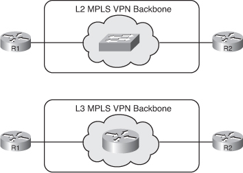
![]() The Layer 2 MPLS VPN provides a Layer 2 service across the backbone, where Routers R1 and R2 are connected together on the same IP subnet. Figure 2-28 represents connectivity through the backbone as a Layer 2 switch.
The Layer 2 MPLS VPN provides a Layer 2 service across the backbone, where Routers R1 and R2 are connected together on the same IP subnet. Figure 2-28 represents connectivity through the backbone as a Layer 2 switch.
![]() The Layer 3 MPLS VPN provides a Layer 3 service across the backbone, where Routers R1 and R2 are connected to ISP edge routers. On each side, a separate IP subnet is used. Figure 2-28 represents connectivity through the backbone as a router.
The Layer 3 MPLS VPN provides a Layer 3 service across the backbone, where Routers R1 and R2 are connected to ISP edge routers. On each side, a separate IP subnet is used. Figure 2-28 represents connectivity through the backbone as a router.
![]() The following sections describe Layer 3 and Layer 2 MPLS VPNs.
The following sections describe Layer 3 and Layer 2 MPLS VPNs.
Layer 3 MPLS VPNs
![]() This section describes Layer 3 MPLS VPNs and how EIGRP is deployed over them.
This section describes Layer 3 MPLS VPNs and how EIGRP is deployed over them.
Layer 3 MPLS VPN Overview
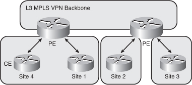
![]() As shown in Figure 2-29, in MPLS VPN terminology, the network is divided into the customer-controlled part (the C-network) and the provider-controlled part (the P-network). Contiguous portions of C-network are called sites and are linked to the P-network via customer edge routers (CE routers). The CE routers are connected to the provider edge (PE) routers, which serve as the edge devices of the Provider network. The core devices in the Provider network (the P-routers) provide the transport across the provider backbone and do not carry customer routes. The service provider connects multiple customers over a common MPLS backbone using MPLS VPNs.
As shown in Figure 2-29, in MPLS VPN terminology, the network is divided into the customer-controlled part (the C-network) and the provider-controlled part (the P-network). Contiguous portions of C-network are called sites and are linked to the P-network via customer edge routers (CE routers). The CE routers are connected to the provider edge (PE) routers, which serve as the edge devices of the Provider network. The core devices in the Provider network (the P-routers) provide the transport across the provider backbone and do not carry customer routes. The service provider connects multiple customers over a common MPLS backbone using MPLS VPNs.


![]() The architecture of a PE router in an MPLS VPN is similar to the architecture of a point of presence (POP) in a dedicated PE router peer-to-peer model; however, in an MPLS VPN, the whole architecture is condensed into one physical device. In an MPLS VPN, each customer is assigned an independent routing table—the virtual routing and forwarding (VRF) table in the PE router—that corresponds to the dedicated PE router in a traditional peer-to-peer model. Routing across the provider backbone is performed by a separate routing process that uses a global IP routing table. This routing process corresponds to the P-routers within the in traditional peer-to-peer model.
The architecture of a PE router in an MPLS VPN is similar to the architecture of a point of presence (POP) in a dedicated PE router peer-to-peer model; however, in an MPLS VPN, the whole architecture is condensed into one physical device. In an MPLS VPN, each customer is assigned an independent routing table—the virtual routing and forwarding (VRF) table in the PE router—that corresponds to the dedicated PE router in a traditional peer-to-peer model. Routing across the provider backbone is performed by a separate routing process that uses a global IP routing table. This routing process corresponds to the P-routers within the in traditional peer-to-peer model.
![]() The MPLS VPN backbone in Figure 2-29 is a Layer 3 backbone. The CE routers treat the PE routers the same as they treat other customer routers in the path between sites. PE routers maintain separate routing tables for each customer.
The MPLS VPN backbone in Figure 2-29 is a Layer 3 backbone. The CE routers treat the PE routers the same as they treat other customer routers in the path between sites. PE routers maintain separate routing tables for each customer.
![]() The MPLS VPN architecture provides ISPs with a peer-to-peer VPN architecture that combines the best features of an overlay VPN (including support for overlapping customer address spaces) with the best features of peer-to-peer VPNs, including the following:
The MPLS VPN architecture provides ISPs with a peer-to-peer VPN architecture that combines the best features of an overlay VPN (including support for overlapping customer address spaces) with the best features of peer-to-peer VPNs, including the following:
Customer Perspective of Layer 3 MPLS VPNs
![]() As illustrated in Figure 2-30, the MPLS VPN backbone looks like a standard corporate backbone to the CE routers. The CE routers run standard IP routing software and exchange routing updates with the PE routers, which appear to them as normal routers in the customer’s network. Therefore, the customer and the SP must agree on EIGRP parameters.
As illustrated in Figure 2-30, the MPLS VPN backbone looks like a standard corporate backbone to the CE routers. The CE routers run standard IP routing software and exchange routing updates with the PE routers, which appear to them as normal routers in the customer’s network. Therefore, the customer and the SP must agree on EIGRP parameters.
![]() The internal topology of the MPLS backbone is transparent to the customer. The internal P-routers are hidden from the customer’s view and the CE routers are unaware of the MPLS VPN.
The internal topology of the MPLS backbone is transparent to the customer. The internal P-routers are hidden from the customer’s view and the CE routers are unaware of the MPLS VPN.
![]() In a Layer 3 MPLS VPN, the following requirements must be met:
In a Layer 3 MPLS VPN, the following requirements must be met:
- The customer routers (the CE routers) should not be MPLS VPN aware. They should run standard IP routing software.
- The provider core routers (the P-routers) must not carry customer (VPN) routes, to make the MPLS VPN solution scalable.
- The PE routers must support MPLS VPN services and traditional IP services.
EIGRP over Layer 3 MPLS VPN
![]() Figure 2-31 provides an example of EIGRP deployed over a Layer 3 MPLS VPN. The configurations for Routers R1 and R2 are shown in Example 2-39.
Figure 2-31 provides an example of EIGRP deployed over a Layer 3 MPLS VPN. The configurations for Routers R1 and R2 are shown in Example 2-39.


interface FastEthernet0/0
ip address 192.168.1.2 255.255.255.252
!
router eigrp 110
network 172.16.1.0 0.0.0.255
network 192.168.1.0
R2#
interface FastEthernet0/0
ip address 192.168.2.2 255.255.255.252
!
router eigrp 110
network 172.17.2.0 0.0.0.255
network 192.168.2.0
![]() Routers R1 and R2 are configured for EIGRP as if there were a corporate core network between them. The customer has to agree on the EIGRP parameters (such as the autonomous system number, authentication password, and so on) with the SP to ensure connectivity. The SP often governs these parameters.
Routers R1 and R2 are configured for EIGRP as if there were a corporate core network between them. The customer has to agree on the EIGRP parameters (such as the autonomous system number, authentication password, and so on) with the SP to ensure connectivity. The SP often governs these parameters.
![]() The PE routers receive routing updates from the CE routers and install these updates in the appropriate VRF table. This part of the configuration and operation is the SP’s responsibility.
The PE routers receive routing updates from the CE routers and install these updates in the appropriate VRF table. This part of the configuration and operation is the SP’s responsibility.
![]() Example 2-40 displays the resulting EIGRP neighbor tables on the R1 and R2 routers. Notice that Router R1 establishes an EIGRP neighbor relationship with the PE1 router, and Router R2 establishes an EIGRP neighbor relationship with the PE2 router. Routers R1 and R2 do not establish an EIGRP neighbor relationship with each other.
Example 2-40 displays the resulting EIGRP neighbor tables on the R1 and R2 routers. Notice that Router R1 establishes an EIGRP neighbor relationship with the PE1 router, and Router R2 establishes an EIGRP neighbor relationship with the PE2 router. Routers R1 and R2 do not establish an EIGRP neighbor relationship with each other.
IP-EIGRP neighbors for process 110
H Address Interface Hold Uptime SRTT RTO Q Seq
(sec) (ms) Cnt Num
0 192.168.1.1 Fe0/0 10 00:07:22 10 2280 0 5
R2#show ip eigrp neighbors
IP-EIGRP neighbors for process 110
H Address Interface Hold Uptime SRTT RTO Q Seq
(sec) (ms) Cnt Num
0 192.168.2.1 Fe0/0 10 00:17:02 10 1380 0 5
Layer 2 MPLS VPNs
![]() This section describes Layer 2 MPLS VPNs and how EIGRP is deployed over them.
This section describes Layer 2 MPLS VPNs and how EIGRP is deployed over them.
Ethernet Port-to-Port Connectivity over a Layer 2 MPLS VPN
![]() With a Layer 2 MPLS VPN, an MPLS backbone provides a Layer 2 Ethernet port-to-port connection, such as between the two customer Routers R1 and R2 in Figure 2-32.
With a Layer 2 MPLS VPN, an MPLS backbone provides a Layer 2 Ethernet port-to-port connection, such as between the two customer Routers R1 and R2 in Figure 2-32.


![]() In Figure 2-32, Routers R1 and R2 are exchanging Ethernet frames. The PE1 router takes the Ethernet frame received from the directly connected Router R1, encapsulates it into an MPLS packet, and forwards it across the backbone to the PE2 router. The PE2 router decapsulates the MPLS packet and reproduces the Ethernet frame on its Ethernet link to Router R2. This process is a type of AToM called EoMPLS. (EoMPLS is also known as a type of Metro Ethernet service.)
In Figure 2-32, Routers R1 and R2 are exchanging Ethernet frames. The PE1 router takes the Ethernet frame received from the directly connected Router R1, encapsulates it into an MPLS packet, and forwards it across the backbone to the PE2 router. The PE2 router decapsulates the MPLS packet and reproduces the Ethernet frame on its Ethernet link to Router R2. This process is a type of AToM called EoMPLS. (EoMPLS is also known as a type of Metro Ethernet service.)
![]() AToM and EoMPLS do not include any MAC layer address learning and filtering. Therefore routers PE1 and PE2 do not filter any frames based on MAC addresses. AToM and EoMPLS also do not use the Spanning Tree Protocol (STP). Bridge protocol data units (BPDUs) are propagated transparently and not processed, so LAN loop detection must be performed by other devices or avoided by design. A service provider can use LAN switches in conjunction with AToM and EoMPLS to provide these features.
AToM and EoMPLS do not include any MAC layer address learning and filtering. Therefore routers PE1 and PE2 do not filter any frames based on MAC addresses. AToM and EoMPLS also do not use the Spanning Tree Protocol (STP). Bridge protocol data units (BPDUs) are propagated transparently and not processed, so LAN loop detection must be performed by other devices or avoided by design. A service provider can use LAN switches in conjunction with AToM and EoMPLS to provide these features.
![]() In the example in Figure 2-33, Routers R1 and R2 communicate with EIGRP over EoMPLS. The configuration for both routers is shown in Example 2-41.
In the example in Figure 2-33, Routers R1 and R2 communicate with EIGRP over EoMPLS. The configuration for both routers is shown in Example 2-41.


interface FastEthernet0/0
ip address 192.168.1.101 255.255.255.224
!
router eigrp 110
network 172.16.1.0 0.0.0.255
network 192.168.1.0
R2#
interface FastEthernet0/0
ip address 192.168.1.102 255.255.255.224
!
router eigrp 110
network 172.17.2.0 0.0.0.255
network 192.168.1.0
![]() When deploying EIGRP over EoMPLS, there are no changes to the EIGRP configuration from the customer perspective. EIGRP needs to be enabled with the correct autonomous system number (the same on both Routers R1 and R2). The network commands must include all the interfaces that will run EIGRP, including the link toward the PE routers (routers PE1 and PE2) over which the Routers R1 and R2 will form their neighbor relationship. From the EIGRP perspective, the MPLS backbone and routers PE1 and PE2 are not visible. A neighbor relationship is established directly between Routers R1 and R2 over the MPLS backbone, and is displayed using the show ip eigrp neighbors command. Output from this command is shown in Example 2-42.
When deploying EIGRP over EoMPLS, there are no changes to the EIGRP configuration from the customer perspective. EIGRP needs to be enabled with the correct autonomous system number (the same on both Routers R1 and R2). The network commands must include all the interfaces that will run EIGRP, including the link toward the PE routers (routers PE1 and PE2) over which the Routers R1 and R2 will form their neighbor relationship. From the EIGRP perspective, the MPLS backbone and routers PE1 and PE2 are not visible. A neighbor relationship is established directly between Routers R1 and R2 over the MPLS backbone, and is displayed using the show ip eigrp neighbors command. Output from this command is shown in Example 2-42.
IP-EIGRP neighbors for process 110
H Address Interface Hold Uptime SRTT RTO Q Seq
(sec) (ms) Cnt Num
0 192.168.1.102 Fe0/0 10 00:07:22 10 2280 0 5
R2#show ip eigrp neighbors
IP-EIGRP neighbors for process 110
H Address Interface Hold Uptime SRTT RTO Q Seq
(sec) (ms) Cnt Num
0 192.168.1.101 Fe0/0 10 00:17:02 10 1380 0 5
Ethernet VLAN Connectivity
![]() Figure 2-34 illustrates an alternative scenario in which the two customer Routers R1 and R2 are connected to the MPLS edge routers PE1 and PE2 via VLAN subinterfaces. Different subinterfaces in the PE routers are used to connect to different VLANs. The PE1 subinterface to the VLAN where the Router R1 is connected is used for AToM forwarding. The Ethernet frame that arrives from Router R1 on the specific VLAN subinterface is encapsulated into MPLS and forwarded across the backbone to Router PE2. The PE2 router decapsulates the packet and reproduces the Ethernet frame on its outgoing VLAN subinterface to Router R2.
Figure 2-34 illustrates an alternative scenario in which the two customer Routers R1 and R2 are connected to the MPLS edge routers PE1 and PE2 via VLAN subinterfaces. Different subinterfaces in the PE routers are used to connect to different VLANs. The PE1 subinterface to the VLAN where the Router R1 is connected is used for AToM forwarding. The Ethernet frame that arrives from Router R1 on the specific VLAN subinterface is encapsulated into MPLS and forwarded across the backbone to Router PE2. The PE2 router decapsulates the packet and reproduces the Ethernet frame on its outgoing VLAN subinterface to Router R2.


EIGRP Load Balancing
![]() This section describes EIGRP equal-cost and unequal-cost load balancing.
This section describes EIGRP equal-cost and unequal-cost load balancing.
EIGRP Equal-Cost Load Balancing
![]() Equal-cost load balancing is a router’s capability to distribute traffic over all the routers that have the same metric for the destination address. All IP routing protocols on Cisco routers can perform equal-cost load balancing.
Equal-cost load balancing is a router’s capability to distribute traffic over all the routers that have the same metric for the destination address. All IP routing protocols on Cisco routers can perform equal-cost load balancing.
![]() Notice that the terminology is equal-cost even though the metric used in the routing protocol may not be called cost (as is the case for EIGRP).
Notice that the terminology is equal-cost even though the metric used in the routing protocol may not be called cost (as is the case for EIGRP).
![]() Load balancing increases the utilization of network segments, thus increasing effective network bandwidth.
Load balancing increases the utilization of network segments, thus increasing effective network bandwidth.
![]() By default, the Cisco IOS balances between a maximum of four equal-cost paths for IP. Using the maximum-paths maximum-path router configuration command, you can request that up to 16 equally good routes be kept in the routing table. Set the maximum-path parameter to 1 to disable load balancing. When a packet is process-switched, load balancing over equal-cost paths occurs on a per-packet basis. When packets are fast-switched, load balancing over equal-cost paths is on a per-destination basis.
By default, the Cisco IOS balances between a maximum of four equal-cost paths for IP. Using the maximum-paths maximum-path router configuration command, you can request that up to 16 equally good routes be kept in the routing table. Set the maximum-path parameter to 1 to disable load balancing. When a packet is process-switched, load balancing over equal-cost paths occurs on a per-packet basis. When packets are fast-switched, load balancing over equal-cost paths is on a per-destination basis.
| Note |
|
| Note |
|
![]() Figure 2-35 illustrates an example network with sample metrics indicated (the metrics are smaller than actual values for easier computation in the example). Example 2-43 shows the EIGRP configuration on Router R1. Table 2-7 displays the contents of Router R1’s topology table for the 172.16.2.0/24 route.
Figure 2-35 illustrates an example network with sample metrics indicated (the metrics are smaller than actual values for easier computation in the example). Example 2-43 shows the EIGRP configuration on Router R1. Table 2-7 displays the contents of Router R1’s topology table for the 172.16.2.0/24 route.


|
|
|
|
|
|---|---|---|---|
|
|
|
|
|
|
|
|
| |
|
|
|
| |
|
|
|
|
network 172.16.1.0 0.0.0.255
network 192.168.1.0
network 192.168.2.0
network 192.168.3.0
network 192.168.4.0
maximum–paths 3
![]() Router R1 is configured to support up to three equal-cost paths. Router R1 will keep the routes via R2, R3, and R4 in its routing table because the three paths have the same metric of 40 (they are equal cost), as shown in the FD column in Table 2-7. The path through router R5 is not used because the metric is bigger than 40 (it is 60). Even if this metric were the same as the others, only three of the four routes would be used because of the maximum-paths 3 command.
Router R1 is configured to support up to three equal-cost paths. Router R1 will keep the routes via R2, R3, and R4 in its routing table because the three paths have the same metric of 40 (they are equal cost), as shown in the FD column in Table 2-7. The path through router R5 is not used because the metric is bigger than 40 (it is 60). Even if this metric were the same as the others, only three of the four routes would be used because of the maximum-paths 3 command.
EIGRP Unequal-Cost Load Balancing
![]() EIGRP can also balance traffic across multiple routes that have different metrics—this is called unequal-cost load balancing.
EIGRP can also balance traffic across multiple routes that have different metrics—this is called unequal-cost load balancing.
![]() The degree to which EIGRP performs load balancing is controlled by the variance multiplier router configuration command. The multiplier is a variance value, between 1 and 128, used for load balancing. The default is 1, which means equal-cost load balancing. The multiplier defines the range of metric values that are accepted for load balancing. Setting a variance value greater than 1 allows EIGRP to install multiple loop-free routes with unequal cost in the routing table. EIGRP will always install successors (the best routes) in the routing table. The variance allows feasible successors to also be installed in the routing table.
The degree to which EIGRP performs load balancing is controlled by the variance multiplier router configuration command. The multiplier is a variance value, between 1 and 128, used for load balancing. The default is 1, which means equal-cost load balancing. The multiplier defines the range of metric values that are accepted for load balancing. Setting a variance value greater than 1 allows EIGRP to install multiple loop-free routes with unequal cost in the routing table. EIGRP will always install successors (the best routes) in the routing table. The variance allows feasible successors to also be installed in the routing table.
![]() Only paths that are feasible can be used for load balancing, and the routing table only includes feasible paths. The two feasibility conditions are as follows:
Only paths that are feasible can be used for load balancing, and the routing table only includes feasible paths. The two feasibility conditions are as follows:
- The route must be loop free. As noted earlier, this means that the best metric (the AD) learned from the next router must be less than the local best metric (the current FD). In other words, the next router in the path must be closer to the destination than the current router.
- The metric of the entire path (the FD of the alternative route) must be lower than the variance multiplied by the local best metric (the current FD). In other words, the metric for the entire alternate path must be within the variance.
![]() If both of these conditions are met, the route is called feasible and can be added to the routing table.
If both of these conditions are met, the route is called feasible and can be added to the routing table.
![]() The default value for the EIGRP variance is 1, which indicates equal-cost load balancing. In this case, only routes with the same metric as the successor are installed in the local routing table. The variance command does not limit the maximum number of paths. Instead, it defines the range of metric values that are accepted for load balancing by the EIGRP process. If the variance is set to 2, any EIGRP-learned route with a metric less than two times the successor metric will be installed in the local routing table. For example, if the variance command allows EIGRP to install nine paths and the maximum-path command sets the maximum paths value to 3, just the first three paths out of the available nine will be in the IP routing table.
The default value for the EIGRP variance is 1, which indicates equal-cost load balancing. In this case, only routes with the same metric as the successor are installed in the local routing table. The variance command does not limit the maximum number of paths. Instead, it defines the range of metric values that are accepted for load balancing by the EIGRP process. If the variance is set to 2, any EIGRP-learned route with a metric less than two times the successor metric will be installed in the local routing table. For example, if the variance command allows EIGRP to install nine paths and the maximum-path command sets the maximum paths value to 3, just the first three paths out of the available nine will be in the IP routing table.
| Note |
|
![]() To control how traffic is distributed among routes when multiple routes exist for the same destination network and they have different metrics, use the traffic-share [balanced | min across-interfaces] router configuration command. With the keyword balanced (the default behavior), the router distributes traffic proportionately to the ratios of the metrics associated with the different routes. With the min across-interfaces option, the router uses only routes that have minimum costs. (In other words, all routes that are feasible and within the variance are kept in the routing table, but only those with the minimum cost are used.) This latter option allows feasible backup routes to always be in the routing table, but only be used if the primary route becomes unavailable so that it is no longer in the routing table.
To control how traffic is distributed among routes when multiple routes exist for the same destination network and they have different metrics, use the traffic-share [balanced | min across-interfaces] router configuration command. With the keyword balanced (the default behavior), the router distributes traffic proportionately to the ratios of the metrics associated with the different routes. With the min across-interfaces option, the router uses only routes that have minimum costs. (In other words, all routes that are feasible and within the variance are kept in the routing table, but only those with the minimum cost are used.) This latter option allows feasible backup routes to always be in the routing table, but only be used if the primary route becomes unavailable so that it is no longer in the routing table.
![]() Figure 2-36 illustrates the same network as in Figure 2-35, but with modified metrics. Example 2-44 shows the command added to the R1 router, setting the variance to 2. Table 2-8 displays the new topology table on the R1 router for the 172.16.2.0/24 route.
Figure 2-36 illustrates the same network as in Figure 2-35, but with modified metrics. Example 2-44 shows the command added to the R1 router, setting the variance to 2. Table 2-8 displays the new topology table on the R1 router for the 172.16.2.0/24 route.


|
|
|
| |
|---|---|---|---|
|
|
|
|
|
|
|
|
| |
|
|
|
| |
|
|
|
|
variance 2
![]() Router R1 uses Router R3 as the successor because its FD is lowest (20). With the variance 2 command applied to Router R1, the path through Router R2 meets the criteria for load balancing. In this case, the FD through Router R2 (30) is less than twice the FD through the successor Router R3 (2 * 20 = 40).
Router R1 uses Router R3 as the successor because its FD is lowest (20). With the variance 2 command applied to Router R1, the path through Router R2 meets the criteria for load balancing. In this case, the FD through Router R2 (30) is less than twice the FD through the successor Router R3 (2 * 20 = 40).
![]() Router R4 is not considered for load balancing because the FD through Router R4 (45) is greater than twice the FD for the successor (Router R3) (2 * 20 = 40). In this example, however, Router R4 would never be an FS no matter what the variance is, because its AD of 25 is greater than Router R1’s FD of 20. Therefore, to avoid a potential routing loop, Router R4 is not considered closer to the destination than Router R1 and cannot be an FS.
Router R4 is not considered for load balancing because the FD through Router R4 (45) is greater than twice the FD for the successor (Router R3) (2 * 20 = 40). In this example, however, Router R4 would never be an FS no matter what the variance is, because its AD of 25 is greater than Router R1’s FD of 20. Therefore, to avoid a potential routing loop, Router R4 is not considered closer to the destination than Router R1 and cannot be an FS.
![]() Router R5 is not considered for load balancing with this variance because the FD through router R5 (50) is more than twice the FD for the successor through Router R3 (2 * 20 = 40). In this example, however, router R5 would be an FS because router R5’s AD of 10 is lower than Router R3’s FD of 20.
Router R5 is not considered for load balancing with this variance because the FD through router R5 (50) is more than twice the FD for the successor through Router R3 (2 * 20 = 40). In this example, however, router R5 would be an FS because router R5’s AD of 10 is lower than Router R3’s FD of 20.
![]() The load in Figure 2-36 is balanced proportional to the bandwidth. The FD of the route via Router R2 is 30, and the FD of the route via Router R3 is 20. The ratio of traffic between the two paths (via R2 : via R3) is therefore 3/5 : 2/5.
The load in Figure 2-36 is balanced proportional to the bandwidth. The FD of the route via Router R2 is 30, and the FD of the route via Router R3 is 20. The ratio of traffic between the two paths (via R2 : via R3) is therefore 3/5 : 2/5.
![]() In another example of unequal load balancing, four paths to a destination have the following metrics:
In another example of unequal load balancing, four paths to a destination have the following metrics:
- Path 1: 1100
- Path 2: 1100
- Path 3: 2000
- Path 4: 4000
![]() By default, the router routes to the destination using both Paths 1 and 2 because they have the same metric. Assuming no potential routing loops exist, the variance 2 command would load balance over Paths 1, 2, and 3, because 1100 * 2 = 2200, which is greater than the metric through Path 3. Similarly, the variance 4 command would also include Path 4.
By default, the router routes to the destination using both Paths 1 and 2 because they have the same metric. Assuming no potential routing loops exist, the variance 2 command would load balance over Paths 1, 2, and 3, because 1100 * 2 = 2200, which is greater than the metric through Path 3. Similarly, the variance 4 command would also include Path 4.
EIGRP Bandwidth Use Across WAN Links
![]() As discussed earlier, EIGRP operates efficiently in WAN environments and is scalable on both point-to-point links and NBMA multipoint and point-to-point links. Because of the inherent differences in links’ operational characteristics, default configuration of WAN connections might not be optimal. A solid understanding of EIGRP operation coupled with knowledge of link speeds can yield an efficient, reliable, scalable router configuration.
As discussed earlier, EIGRP operates efficiently in WAN environments and is scalable on both point-to-point links and NBMA multipoint and point-to-point links. Because of the inherent differences in links’ operational characteristics, default configuration of WAN connections might not be optimal. A solid understanding of EIGRP operation coupled with knowledge of link speeds can yield an efficient, reliable, scalable router configuration.
![]() This section first introduces how EIGRP uses the bandwidth on interfaces, and then provides examples of EIGRP on various WANs.
This section first introduces how EIGRP uses the bandwidth on interfaces, and then provides examples of EIGRP on various WANs.
EIGRP Link Utilization
![]() By default, EIGRP uses up to 50 percent of the bandwidth declared on an interface or subinterface. EIGRP uses the bandwidth of the link set by the bandwidth command, or the link’s default bandwidth if none is configured, when calculating how much bandwidth to use.
By default, EIGRP uses up to 50 percent of the bandwidth declared on an interface or subinterface. EIGRP uses the bandwidth of the link set by the bandwidth command, or the link’s default bandwidth if none is configured, when calculating how much bandwidth to use.
![]() You can adjust this percentage on an interface or subinterface with the ip bandwidth-percent eigrp as-number percent interface configuration command. The as-number is the EIGRP autonomous system number. The percent parameter is the percentage of the configured bandwidth that EIGRP can use. You can set the percentage to a value greater than 100, which might be useful if the bandwidth is configured artificially low for routing policy reasons. Example 2-45 shows a configuration that allows EIGRP to use 40 kbps (200 percent of the configured bandwidth, 20 kbps) on the interface. It is essential to make sure that the line is provisioned to handle the configured capacity. (The next section, “Examples of EIGRP on WANs,” provides some more examples of when this command is useful.)
You can adjust this percentage on an interface or subinterface with the ip bandwidth-percent eigrp as-number percent interface configuration command. The as-number is the EIGRP autonomous system number. The percent parameter is the percentage of the configured bandwidth that EIGRP can use. You can set the percentage to a value greater than 100, which might be useful if the bandwidth is configured artificially low for routing policy reasons. Example 2-45 shows a configuration that allows EIGRP to use 40 kbps (200 percent of the configured bandwidth, 20 kbps) on the interface. It is essential to make sure that the line is provisioned to handle the configured capacity. (The next section, “Examples of EIGRP on WANs,” provides some more examples of when this command is useful.)
Router(config-if)#bandwidth 20
Router(config-if)#ip bandwidth-percent eigrp 1 200
![]() The Cisco IOS assumes that point-to-point Frame Relay subinterfaces are operating at the default speed of the interface. In many implementations, however, only fractional speeds (such as a fractional T1) are available. Therefore, when configuring these subinterfaces, set the bandwidth to match the contracted CIR.
The Cisco IOS assumes that point-to-point Frame Relay subinterfaces are operating at the default speed of the interface. In many implementations, however, only fractional speeds (such as a fractional T1) are available. Therefore, when configuring these subinterfaces, set the bandwidth to match the contracted CIR.
![]() When configuring multipoint interfaces (especially for Frame Relay, but also for ATM and ISDN PRI), remember that the bandwidth is shared equally by all neighbors. That is, EIGRP uses the bandwidth command on the physical interface divided by the number of Frame Relay neighbors connected on that physical interface to get the bandwidth attributed to each neighbor. EIGRP configuration should reflect the correct percentage of the actual available bandwidth on the line.
When configuring multipoint interfaces (especially for Frame Relay, but also for ATM and ISDN PRI), remember that the bandwidth is shared equally by all neighbors. That is, EIGRP uses the bandwidth command on the physical interface divided by the number of Frame Relay neighbors connected on that physical interface to get the bandwidth attributed to each neighbor. EIGRP configuration should reflect the correct percentage of the actual available bandwidth on the line.
![]() Each installation has a unique topology, and with that comes unique configurations. Differing CIR values often require a hybrid configuration that blends the characteristics of point-to-point circuits with multipoint circuits. When configuring multipoint interfaces, configure the bandwidth to represent the minimum CIR times the number of circuits. This approach might not fully use the higher-speed circuits, but it ensures that the circuits with the lowest CIR will not be overdriven. If the topology has a small number of very low-speed circuits, these interfaces are typically defined as point-to-point so that their bandwidth can be set to match the provisioned CIR.
Each installation has a unique topology, and with that comes unique configurations. Differing CIR values often require a hybrid configuration that blends the characteristics of point-to-point circuits with multipoint circuits. When configuring multipoint interfaces, configure the bandwidth to represent the minimum CIR times the number of circuits. This approach might not fully use the higher-speed circuits, but it ensures that the circuits with the lowest CIR will not be overdriven. If the topology has a small number of very low-speed circuits, these interfaces are typically defined as point-to-point so that their bandwidth can be set to match the provisioned CIR.
Examples of EIGRP on WANs
![]() In Figure 2-37, Router C’s interface has been configured for a bandwidth of 224 kbps. Four neighbors exist in this multipoint topology, so each circuit is allocated one-quarter of the configured bandwidth on the interface, resulting in 224 / 4 = 56 kbps allocated per circuit. This 56-kbps allocation matches the provisioned CIR of each circuit.
In Figure 2-37, Router C’s interface has been configured for a bandwidth of 224 kbps. Four neighbors exist in this multipoint topology, so each circuit is allocated one-quarter of the configured bandwidth on the interface, resulting in 224 / 4 = 56 kbps allocated per circuit. This 56-kbps allocation matches the provisioned CIR of each circuit.
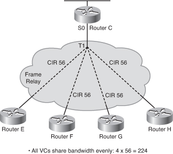
![]() Example 2-46 shows the configuration for Router C’s Serial 0 interface.
Example 2-46 shows the configuration for Router C’s Serial 0 interface.
RouterC(config-if)#encapsulation frame-relay
RouterC(config-if)#bandwidth 224
![]() In Figure 2-38, one circuit has been provisioned for a 56-kbps CIR, and the other three circuits have a higher CIR of 256 kbps. The interface on Router C has been configured for a bandwidth equal to the lowest CIR multiplied by the number of circuits being supported (56 * 4 = 224), as shown in Example 2-47. This configuration protects against overwhelming the slowest-speed circuit in the topology.
In Figure 2-38, one circuit has been provisioned for a 56-kbps CIR, and the other three circuits have a higher CIR of 256 kbps. The interface on Router C has been configured for a bandwidth equal to the lowest CIR multiplied by the number of circuits being supported (56 * 4 = 224), as shown in Example 2-47. This configuration protects against overwhelming the slowest-speed circuit in the topology.
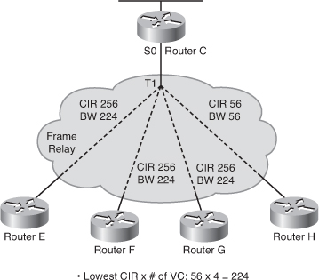
RouterC(config-if)#encapsulation frame-relay
RouterC(config-if)#bandwidth 224
![]() Figure 2-39 presents a hybrid solution to this network.
Figure 2-39 presents a hybrid solution to this network.
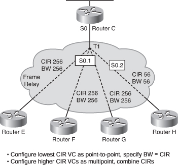
![]() Example 2-48 shows the configuration applied to Router C in Figure 2-39.
Example 2-48 shows the configuration applied to Router C in Figure 2-39.
RouterC(config-subif)#bandwidth 768
RouterC(config-subif)#exit
RouterC(config)#interface serial 0.2 point-to-point
RouterC(config-subif)#bandwidth 56
![]() Example 2-48 shows the low-speed circuit configured as point-to-point. The remaining circuits are designated as multipoint, and their respective CIRs are added up to set the interface’s bandwidth (256 + 256 + 256 = 768). On the multipoint interface, the bandwidth is shared equally among all circuits. Thus, the bandwidth will be split into three, with 256 kbps allocated to each circuit.
Example 2-48 shows the low-speed circuit configured as point-to-point. The remaining circuits are designated as multipoint, and their respective CIRs are added up to set the interface’s bandwidth (256 + 256 + 256 = 768). On the multipoint interface, the bandwidth is shared equally among all circuits. Thus, the bandwidth will be split into three, with 256 kbps allocated to each circuit.
![]() Figure 2-40 illustrates a common hub-and-spoke oversubscribed topology with 10 VCs to the remote sites. (Only 4 of the 10 remote sites are shown in the figure.) Example 2-49 shows the configuration used on Routers C and G of Figure 2-40.
Figure 2-40 illustrates a common hub-and-spoke oversubscribed topology with 10 VCs to the remote sites. (Only 4 of the 10 remote sites are shown in the figure.) Example 2-49 shows the configuration used on Routers C and G of Figure 2-40.
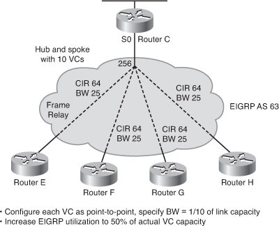
RouterC(config-subif)#bandwidth 25
RouterC(config-subif)#ip bandwidth-percent eigrp 63 128
![]() The circuits are provisioned as 64-kbps links, but there is insufficient bandwidth on Router C (the hub) to support the allocation. For example, if the hub tries to communicate to all remote sites at the same time, the bandwidth that is required exceeds the available link speed of 256 kbps for the hub—10 times the CIR of 64 kbps equals 640 kbps. In a point-to-point topology, all VCs are treated equally and are therefore configured for exactly one-tenth of the available link speed (25 kbps). (Alternatively the Serial 0 main interface could be configured with the bandwidth 256 command.)
The circuits are provisioned as 64-kbps links, but there is insufficient bandwidth on Router C (the hub) to support the allocation. For example, if the hub tries to communicate to all remote sites at the same time, the bandwidth that is required exceeds the available link speed of 256 kbps for the hub—10 times the CIR of 64 kbps equals 640 kbps. In a point-to-point topology, all VCs are treated equally and are therefore configured for exactly one-tenth of the available link speed (25 kbps). (Alternatively the Serial 0 main interface could be configured with the bandwidth 256 command.)
![]() As mentioned, by default EIGRP uses 50 percent of a circuit’s configured bandwidth. EIGRP configuration should reflect the correct percentage of the actual available bandwidth on the line. Therefore, in an attempt to ensure that EIGRP packets are delivered through the Frame Relay network in Figure 2-40, each subinterface has the EIGRP allocation percentage raised to 128 percent of the specified bandwidth. This adjustment causes EIGRP packets to receive approximately 32 kbps of the provisioned 64 kbps on each circuit (because 128% of 25 kbps is 32 kbps). This extra configuration restores the 50-50 ratio that was tampered with when the bandwidth was set to an artificially low value. If the number of VCs changes, these calculations and configurations must be redone.
As mentioned, by default EIGRP uses 50 percent of a circuit’s configured bandwidth. EIGRP configuration should reflect the correct percentage of the actual available bandwidth on the line. Therefore, in an attempt to ensure that EIGRP packets are delivered through the Frame Relay network in Figure 2-40, each subinterface has the EIGRP allocation percentage raised to 128 percent of the specified bandwidth. This adjustment causes EIGRP packets to receive approximately 32 kbps of the provisioned 64 kbps on each circuit (because 128% of 25 kbps is 32 kbps). This extra configuration restores the 50-50 ratio that was tampered with when the bandwidth was set to an artificially low value. If the number of VCs changes, these calculations and configurations must be redone.
0 comments
Post a Comment